| Japanese | English |
14th LSI Design Contests・in Okinawa Design Specification - 3
3.THE COMPRESSION ALGORITHM
In this section we will describe the detail algorithm of DCT/IDCT transform and Quantizer/Dequantizer. The explanation starts from 1D-DCT, and then continues to represent 2D-DCT from 1D-DCT.
3.1. THE ONE-DIMENSIONAL DISCRETE COSINE TRANSFORM (1D-DCT)
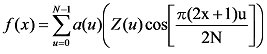
The equation for one-dimension N points DCT is as follows:
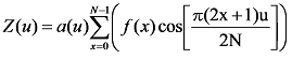
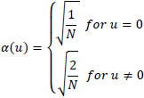
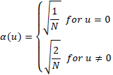
for u=0,1,2 ... N. where α(u) is defined as
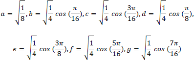
It is clear that for u=0, we will have
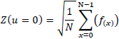
Thus, the first DCT coefficient is the average value of the sample sequence. This value is called DC coefficient and all others values are called AC coefficients.
The above equation can be treated as a matrix multiplication.
where X is input matrix, C is transformation matrix, and Z is transformed matrix. For 8x8 points 1D-DCT, we will have transformation matrix as Equation 5.
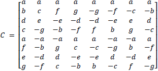
where
3.2. THE ONE-DIMENSIONAL INVERSE DISCRETE COSINE TRANSFORM (1D-IDCT)
Similarly, the inverse transformation is defined as
for x=0,1,2 .... N. α(u) is defined as
The above equation can be treated as matrix multiplication
where X is input matrix, C is transformation matrix, and Z is transformed matrix.
3.3. THE TWO-DIMENSIONAL DCT/IDCT
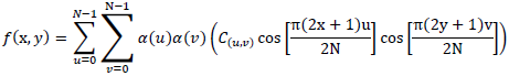
The 2D-DCT is an extension of 1D-DCT and can be defined as
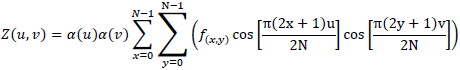
for u,v=0,1,2 .... N-1. α(u) and α(v) are defined in Equation 2.
The inverse transformation is defined as
for x, y = 0,1,2 .... N-1. The 2D-DCT calculation above can be modified using separatility property of DCT equation. Therefore it can be expressed as
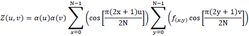
It means that 2D-DCT calculation can be achieved through 1D-DCT horizontal transform (row-wised) and a 1D-DCT vertical transform (column-wised). This idea can be illustrated graphically as shown in Figure 4.
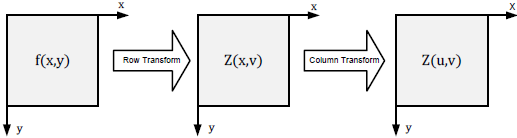
Figure 4. The Computation of 2D-DCT using 1D-DCT
In the matrix operation, 2D-DCT transformation can be calculated using Equation 12
The same idea can be used for inverse DCT, it can expressed as
The importance thing to remember between two stages of 2D-DCT/IDCT Transform, the resulted matrix from previous 1D-DCT (or IDCT) must be transposed before entering to the second stage of 1D-DCT.
3.4. THE QUANTIZATION AND DEQUANTIZATION
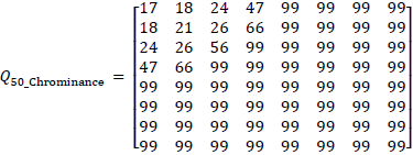
In the quantization process, every element of DCT coefficient is divided by the quantization matrix Q as defined in Equation 14.
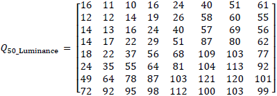
The quantization matrix Q usually has lower number in the upper left and increase as they get closer to the lower right. There is no fixed value of quantization matrix, this is the prerogative of the user to select a quantization matrix. However, JPEG committee has recommended some quantization matrix Q, such the example matrix Q50_Luminance and Q50_Chrominance below.
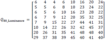
We can customize the compression level at runtime using quantization table which consist of several quantization matrix. If users want to get better compression ratio, they can use higher quantization matrix. But if they want to get better image quality, they can use lower quantization matrix. We can get another quantization matrix by scaling basic quantization matrixes above using Equation 16.
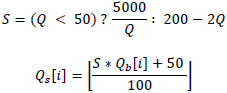
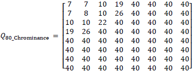
For example, we can scale quantization table for Q80.
At the input of The Decompression Module, we have to Dequantize the DCT coefficients before entering into the IDCT module as defined in Equation 18.。